Physical Computing HS2018
Lecturers: Joël Gähwiler, Luke Franzke
Course Overview
In this course, we will look at physical computing as a method of interaction design. Our definition of Physical Computing refers to the use of hardware and software to make interactive objects that can respond to events in the real world. These events may be general knowledge about the environment (temperature, brightness, etc.) or user interactions (keystroke, approach, touch, etc.). These devices might respond with direct feedback through displays or actuators, or by performing actions in a digital environment. The challenge of physical computing is to make the interface between human and machine as simple and intuitive as possible by taking physical human abilities and habits into account.
Course Goals
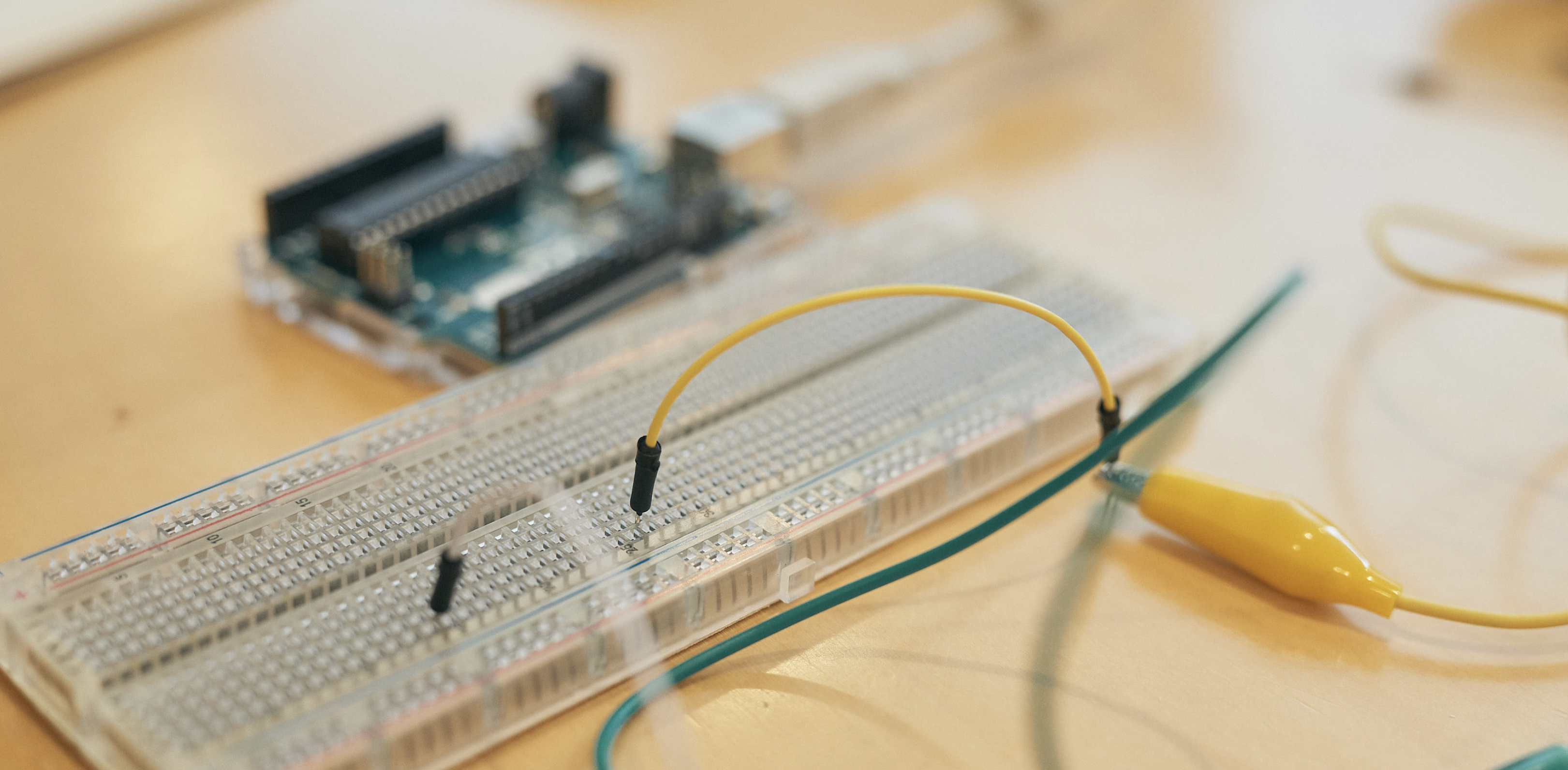
The students learn how to handle hardware and software in order to prototype their own ideas. The students develop an understanding of the characteristics of physical interactions and demonstrate them through functional prototypes. From a technical perspective, students learn the areas of electronics, microcontroller programming (Arduino), sensors and actuators.
In the first one and a half weeks, the students will work individually through the introductory topics. In the second stage, students will form groups of 3 people for the final project.
Topic: Quellen der Energie (im Zauberwald)
This year, students work will be exhibited in Zauberwald in a collective installation. The installation covers the topic of Energy Production and will combine outcomes from Physical Computing and Interactive Visualisation. In the Physical Computing module, students will develop an input device, that will later be used to control a visualisation developed in the Interactive Visualisation module. More information on the project can be found here.
Each input device will be themed on renewable energy sources relating to an energy source in Switzerland. Students will develop the appearance and function of the energy source and build in sensors to allow various forms of interactions from visitors to be fed into the Visualiser.
The available energy sources are:
- Water
- Solar
- Wind
Guidelines for the object:
- Object emits one value from 0.0 to 1.0 to be understood as the current energy production.
- Circular Base with a diameter of 400mm (the tree stump is 600mm).
- Robust, waterproof and resistant in below zero environments.
- Construction only with appropriate materials (decision will be made together).
- The object should have both sensors (inputs) and actuators (feedback).
- Easily reproducible: CAD drawings and electronic schematics must also be delivered.
Technical Specification
Each object must use a Arduino MKR1000 (WiFi, 3.3V) that connects to a shifr.io namespace and transmits the current energy production as string representation of a floating point value between 0.0 and 1.0. At the final presentation we will communicate access credentials to a shared namespace as well as topics for the individual objects that need to be configured. We will use the data to feed a simple visualization that will present the common energy production per power type.
Groups
Wind
- Jennifer, Mara, Felix (wind1)
- Lilian, Randy (wind2)
Water
- Melanie, Marcial, Michelle (water1)
- Duy, Fiona, Colin (water2)
Solar
- Claudia, Stefan, Janina (solar1)
- Andrin, Edna, Dominik (solar2)
Deliverables
Individual
- Scans of Notebook (PDF)
Group
- Final Prototype of Object
- Plans for Final Object
- Drawings (CAD)
- Schematics & Board Layout (Eagle)
- Material List (Spreadsheet)
- Final Presentation
- Standard IAD Documentation
- Video (Making of, Final Prototype)
- Short Documentation (PDF)
Expectations and Grading
Grades will be based on group presentations, class participation, home assignments, documentation (journal) and final work. An attendance of min. 80% is required to pass the course.
- Individual Documentation (30%)
- Group Work (70%)
Presentation
For the presentation you will need to bring your objects to 4.T33. Ensure that your project is connected to shiftr.io using the MKR100 with the shared name space for the Zauberwald project (you will be briefed how to do this). A simple visualisation has been prepared to show the outputs on the screen in the seminar room.
- 5 minutes for presentation, and 5 minutes for feedback and discussion
- Live demonstration of your project
- Explain the process and the thinking that brought you to this outcome
- Indicate any further steps that are required to realise your project in an outdoor, winter setting
- No slides needed
References and Links
Schedule
Morning: 09:00 - 12:00 Uhr, Afternoon: 13:30 - 17:00 Uhr
W1 | Tuesday 9.10 | Wednesday 10.10 | Thursday 11.10 | Friday 12.10 |
|---|---|---|---|---|
| Morning | Kick-off Electricity Basics JG, LF - 4.T06 | Analog Input | Transistors | Digital Components |
| Afternoon | Digital Output | Soldering | ICs, H-Bridges Bits & Atoms III | Individual Work |
W2 | Tuesday 16.10 | Wednesday 17.10 | Thursday 18.10 | Friday 19.10 |
| Morning | EAGLE CAD | Individual Repetition | Ideation | |
| Afternoon | PCB Milling | Networking | Project Kickoff Bits & Atoms III | Concept |
W3 | Tuesday 23.10 | Wednesday 24.10 | Thursday 25.10 | Friday 26.10 |
| Morning | Short Presentation Mentoring | Mentoring | Prototyping | Prototyping |
| Afternoon | Prototyping | Prototyping | Mentoring
| Prototyping |
W4 | Tuesday 30.10 | Wednesday 31.10 | Thursday 01.11 | Friday 02.11 |
| Morning | Build | Build | Build | Bits & Atoms III |
| Afternoon | Mentoring | Build | Final Presentation | Documentation |